Super-resolution Enhancement Evaluation & Downstream Analysis Tutorial (Xenium skin)

This tutorial benchmarks pixel-level imputation results for a Xenium skin panel and illustrates:

1. Spot-level quantitative evaluation: metrics comparing predictions against ground truth.

2. Pixel-level visualization: aligned spatial maps (GT vs CoxFormer vs iStar) for selected genes.

3. Downstream analysis: pixel-level clustering and LIANA-based cell–cell communication (CCC) visualization.

All functions are available in utils/.

0. Configuration

Define the result directory and keep a consistent naming convention for inputs/outputs across all steps.

import warnings
warnings.filterwarnings("ignore")
import os
os.chdir(os.path.abspath(".."))
import scanpy as sc
from utils.Super_resolution_enhancement_utils import evaluate_and_plot, load_pickle, XeniumAlignConfig, plot_xenium_gene_show, plot_spatial_clustering, run_liana_ccc_spatial, plot_liana_lr_dotplot, plot_liana_nmf_spatial

RES_PATH = "Result/Super_resolution_enhancement/skin"
DATA_PATH = "Dataset/Super_resolution_enhancement/skin"
metrics_labels = ["RMSE", "SSIM", "Pearson"]
colors = ["#DBE0ED", "#CC88B0"]
data = {
    "gt": "CoxFormer-Img_pixel_sim_true.npy",
    "pred": {
        "iStar": "iStar_pixel_sim_pred.npy",
        "CoxFormer":  "CoxFormer-Img_pixel_sim_pred.npy",
    }}

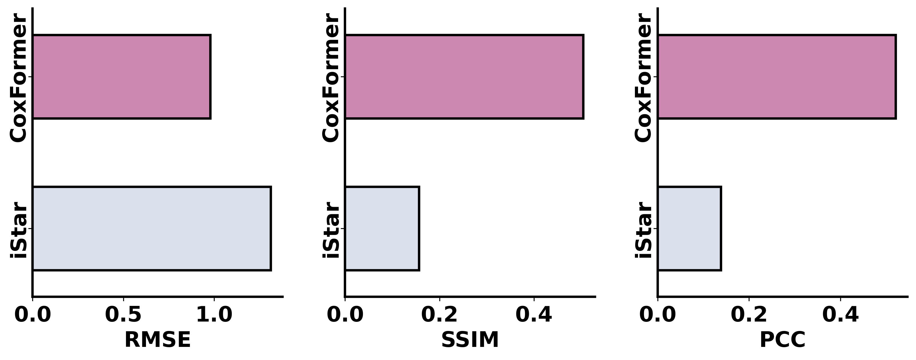
1. Pixel-level evaluation

This section computes and plots pixel-level similarity metrics. Required files under RES_PATH:

• CoxFormer-Img_pixel_sim_true.npy: pixel-level ground truth

• iStar_pixel_sim_pred.npy: iStar prediction

• CoxFormer-Img_pixel_sim_pred.npy: CoxFormer prediction

Output: a summary figure compare_bar_plot.pdf saved under RES_PATH (controlled by out_pdf_name).

metrics_labels = ["RMSE", "SSIM", "PCC"]
metrics = evaluate_and_plot(
    save_dir=RES_PATH,
    data=data,
    metrics_labels=metrics_labels,
    colors=colors,
    out_pdf_name="compare_bar_plot.pdf",
)

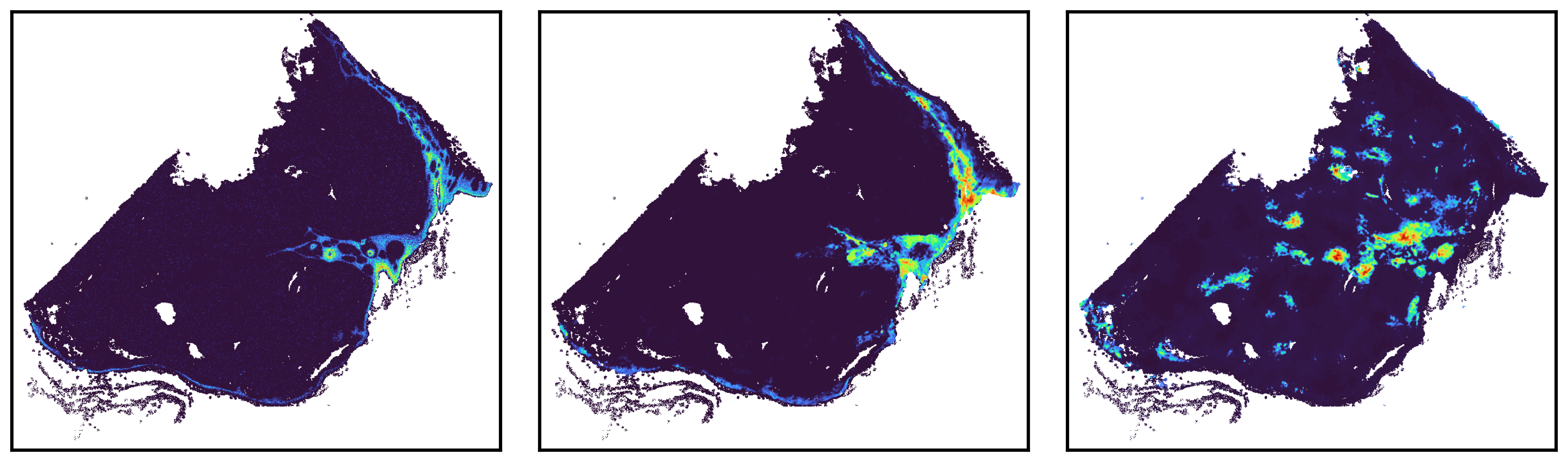
2. Gene-level spatial maps (aligned Xenium panel)

This section loads pixel-level gene dictionaries and renders aligned spatial maps with a consistent mask.

Inputs:

• pixel_cnts_sectionB.pickle: ground-truth Xenium pixel counts (from the section B)

• CoxFormer-Img_pixel_sim_hyper.pkl: CoxFormer pixel prediction dictionary

• iStar_pixel_sim_hyper.pkl: iStar pixel prediction dictionary

• mask-cell_sectionB.png: foreground mask for plotting

2.1 Compared with iStar

gene_cnt = load_pickle(os.path.join(DATA_PATH, "pixel_cnts_sectionB.pickle"))
gene_cnt = {k.upper(): v for k, v in gene_cnt.items()}
gene_coxformer = load_pickle(os.path.join(RES_PATH, "CoxFormer-Img_pixel_sim_hyper.pkl"))
gene_istar = load_pickle(os.path.join(RES_PATH, "iStar_pixel_sim_hyper.pkl"))
gene_show = ["DMKN"]
cfg_panel = XeniumAlignConfig(panel_extra_shift=0)
plot_xenium_gene_show(
    gene_show=gene_show,
    sources={"GT": gene_cnt, "CoxFormer": gene_coxformer, "iStar": gene_istar},
    cfg=cfg_panel,
    mask_path= os.path.join(DATA_PATH, "mask-cell_sectionB.png"),
    out_dir=None,
    out_prefix="Hyper",
    show=True,
    )

Image loaded from Dataset/Super_resolution_enhancement/skin/mask-cell_sectionB.png

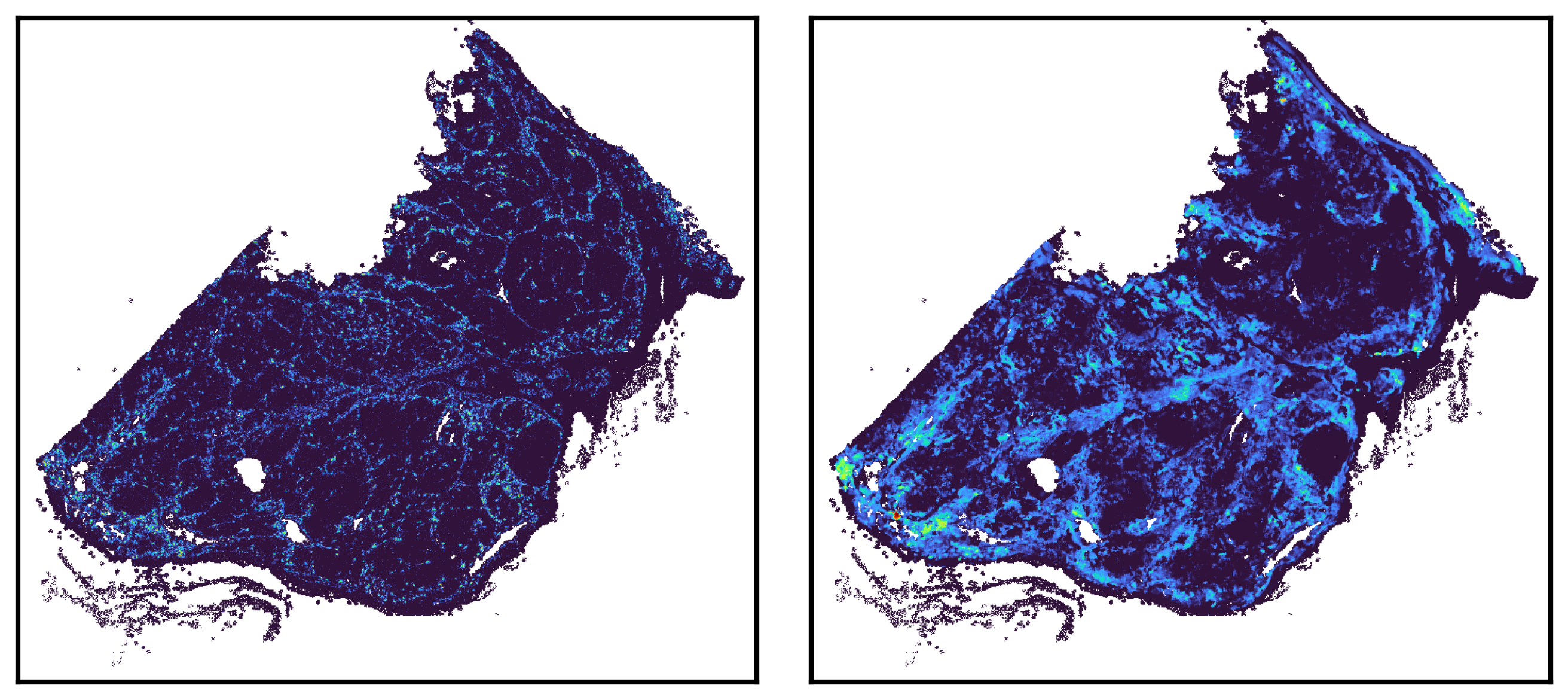
2.2 Compared with Groundtruth (Zero-shot performance)

plot_xenium_gene_show(
     gene_show=["COL6A3"],
     sources={"GT": gene_cnt, "CoxFormer": gene_coxformer},   # 不传 iStar -> 自动两列
     cfg=cfg_panel,
     mask_path= os.path.join(DATA_PATH, "mask-cell_sectionB.png"),
     out_dir=None,
     out_prefix="Hyper_pred",
     show=True,
 )

Image loaded from Dataset/Super_resolution_enhancement/skin/mask-cell_sectionB.png

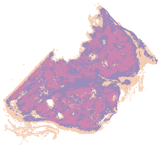
3. Pixel-level clustering and spatial heatmaps

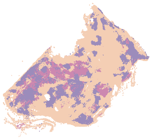
This section clusters pixel-level predicted expression and maps cluster labels back to spatial coordinates. It uses a smaller mask (mask-cell-sub.png) for a focused region.

Outputs: CoxFormer_clustering_heatmap.png and iStar_clustering_heatmap.png saved under save_path.

3.1 Clustering on COPT prediction

mask_png = os.path.join(DATA_PATH, "mask-cell-sub_sectionB.png")
colors = ("#CC88B0", "#F4CEB4", "#9C8CBB")

adata_copt = plot_spatial_clustering(
    pred_pkl_path=os.path.join(RES_PATH, "CoxFormer-Img_pixel_sim_hyper.pkl"),
    mask_png_path=mask_png,
    out_pdf_path=os.path.join(RES_PATH, "CoxFormer_clustering_heatmap.png"),
    n_clusters=3,
    n_pcs=10,
    colors=colors,
)

Image loaded from Dataset/Super_resolution_enhancement/skin/mask-cell-sub_sectionB.png

3.2 Clustering on iStar prediction

# iStar
adata_istar = plot_spatial_clustering(
    pred_pkl_path=os.path.join(RES_PATH, "iStar_pixel_sim_hyper.pkl"),
    mask_png_path=mask_png,
    out_pdf_path=os.path.join(RES_PATH, "iStar_clustering_heatmap.png"),
    n_clusters=3,
    n_pcs=10,
    colors=colors,
)

Image loaded from Dataset/Super_resolution_enhancement/skin/mask-cell-sub_sectionB.png

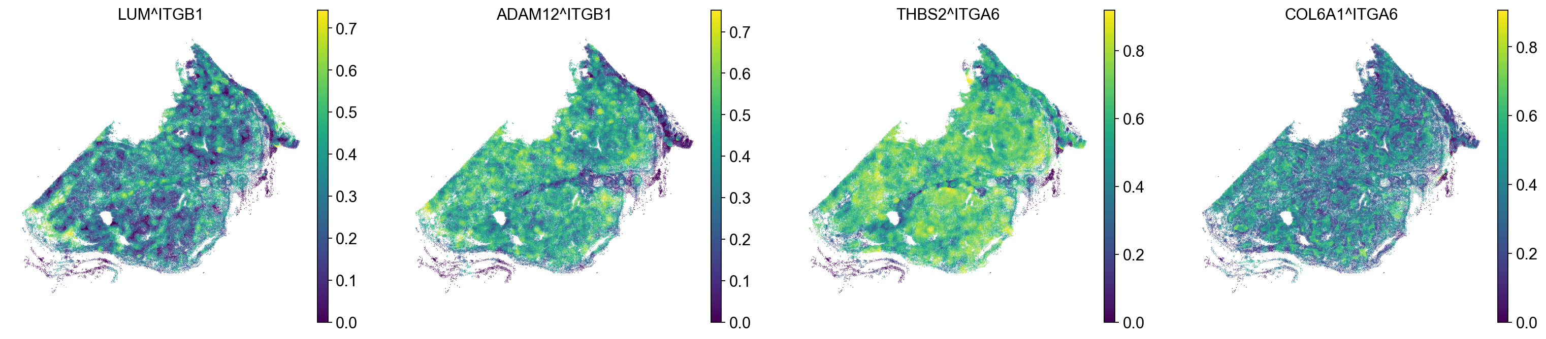
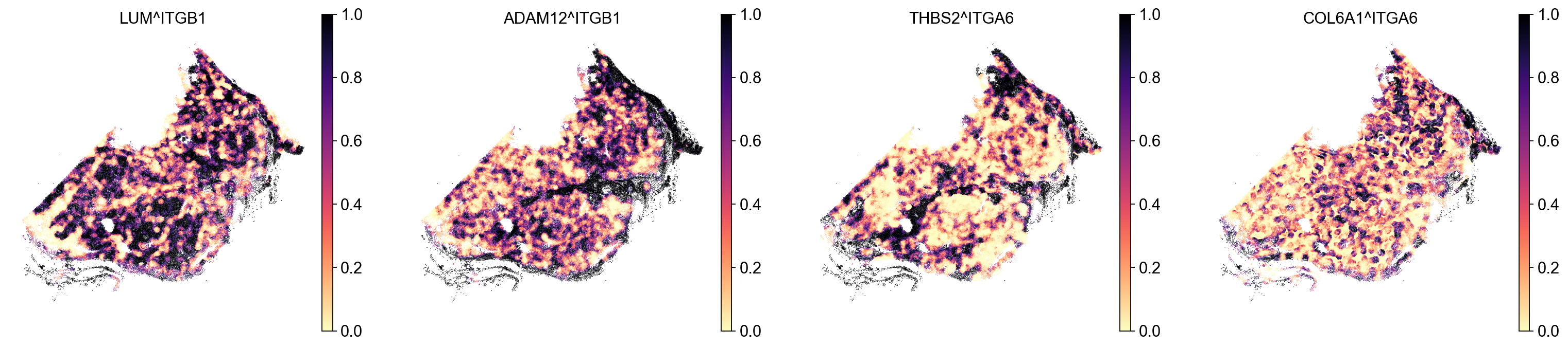
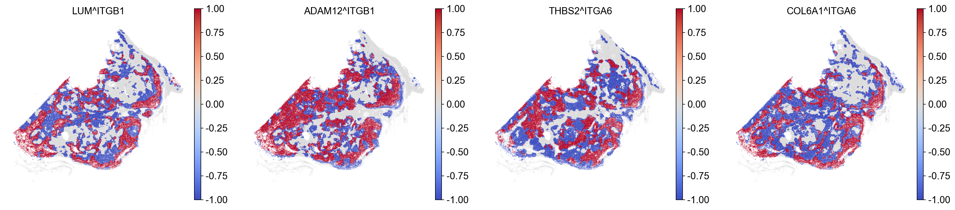
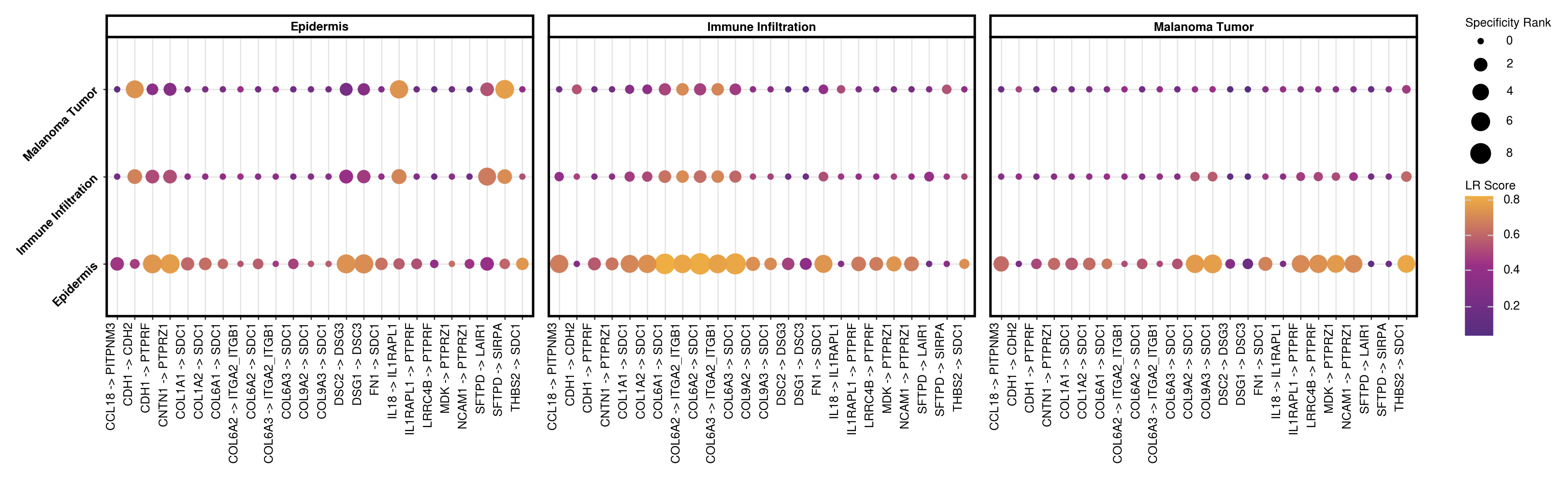
4. Cell–cell communication analysis (LIANA + spatial context)

This section runs LIANA-based CCC inference on the cell-level matrix and visualizes top ligand–receptor interactions and spatial NMF patterns.

4.1 Run CCC inference

adata_base = sc.read_h5ad(os.path.join(DATA_PATH,"cell_matrix.h5ad"))
lrdata_base = run_liana_ccc_spatial(
    adata_base,
    celltype_csv=os.path.join(DATA_PATH, "clusters.csv"),
    coords_csv=os.path.join(DATA_PATH, "cells.csv.gz"),
)

Using `.X`!
Converting to sparse csr matrix!

Using provided `resource`.

0.95 of entities in the resource are missing from the data.

Generating ligand-receptor stats for 106791 samples and 21 features
Assuming that counts were `natural` log-normalized!
Running CellPhoneDB

100%|██████████| 1000/1000 [00:07<00:00, 125.77it/s]

Running Connectome
Running log2FC
Running NATMI
Running SingleCellSignalR

Using `.X`!
Converting to sparse csr matrix!

Using provided `resource`.

100%|██████████| 100/100 [00:04<00:00, 21.52it/s]
100%|██████████| 100/100 [00:13<00:00,  7.43it/s]
... storing 'receptor' as categorical

4.2 Dotplots for ligand–receptor interactions

method = 'CoxFormer'
p = plot_liana_lr_dotplot(os.path.join(RES_PATH, f"cell_cell_communication/lrdata_{method}.h5ad"), method, RES_PATH)
p

4.4 Spatial NMF visualization

method = 'GT'
plot_liana_nmf_spatial(os.path.join(RES_PATH, f"cell_cell_communication/lrdata_{method}.h5ad"), method, RES_PATH, raw_save=False)