Pathological Region Detection Tutorial (CRLM)

This tutorial evaluates spatial gene expression imputation on multiple cancer tissue sections. It illustrates:

1. Section-level visualization: abnormal-region maps and UMAPs derived from model outputs.

2. Gene-level visualization: spatial expression maps for selected marker genes (ground truth vs imputation).

3. Cross-dataset benchmarking: mean±std performance metrics and mean ROC curves aggregated across datasets.

All functions are available in utils/.

0. Configuration

Define the result directory, datasets to benchmark, and a consistent method/color scheme used across all plots.

import warnings
warnings.filterwarnings("ignore")
import os
import pandas as pd
import numpy as np
import scanpy as sc
import matplotlib.pyplot as plt
import matplotlib.colors as mcolors
os.chdir(os.path.abspath(".."))
from utils.Gene_expression_prediction_utils import plot_gene_spatial
from utils.Gene_activity_score_prediction_utils import get_topk_markers, order_spots_by_marker_score, plot_gaussian_heatmap
from utils.Pathological_region_detection_utils import run_cancer_abnormal_benchmark, plot_metrics_barplots, plot_mean_roc, plot_abnormal_region, plot_umap, GO_analysis, plot_go_bubble

datasets = ["CRC1", "CRC2", "LM1", "LM2"]
RES_PATH  = "Result/Pathological_region_detection"
DATA_PATH  = "Dataset/Pathological_region_detection"

colors = ['#E56F5E', '#F19685', '#F6C957', '#FFB77F', '#FBE8D5', '#43978F', '#9EC4BE', '#ABD0F1', '#DCE9F4']
methods = ["CoxFormer", "gimVI", "SpaGE", "SpaOTsc", "Tangram",  "Seurat", "stPlus", "novoSpaRc",  "LIGER"]
color_map = dict(zip(methods, colors))

1. Load ground truth and imputed matrices

This section loads:

• meta.tsv: spot-level metadata (e.g., cluster labels and optional pseudotime)

• cnts.tsv: ground truth gene activity scores matrix (genes × score)

• {tool}_impute.csv: imputed ATAC matrices from different methods

dataset = "CRC1"
locs = pd.read_csv(os.path.join(DATA_PATH, dataset, "locs.tsv"), header=0, sep="\t", index_col=0)
groundtruth = pd.read_csv(os.path.join(RES_PATH,dataset,"groundtruth.csv"), sep=",")
coxformer = pd.read_csv(os.path.join(RES_PATH,dataset,'CoxFormer_impute.csv'),sep=',')

2. Abnormal detection across methods

This section runs the abnormal-region detection procedure for multiple methods. For each method:

1. Load the imputed expression matrix.

2. Apply a unified detection function (e.g., abnormal_detection) using the same inputs and gene ordering.

3. Store the resulting evaluation metrics in a dictionary for later aggregation and plotting.

This step produces method-level metrics and/or intermediate outputs saved under the dataset result directory.

run_cancer_abnormal_benchmark(datasets=datasets, save_dir=RES_PATH, src_dir=DATA_PATH, methods=methods)

==================== CRC1 ====================
--------------- CoxFormer ---------------
Mean absolute expression per cluster: leiden
0    2.175350
1    2.065645
dtype: float64
Cluster with the highest mean absolute expression: 0
ROC_AUC: 0.8603
Precision: 0.8192
Recall: 0.9650
F1-score: 0.8861
Accuracy: 0.8675
--------------- gimVI ---------------
Mean absolute expression per cluster: leiden
0    0.822242
1    0.659776
dtype: float64
Cluster with the highest mean absolute expression: 0
ROC_AUC: 0.7830
Precision: 0.7296
Recall: 0.9847
F1-score: 0.8382
Accuracy: 0.7969
--------------- SpaGE ---------------
Mean absolute expression per cluster: leiden
0    0.094753
1    0.066033
dtype: float64
Cluster with the highest mean absolute expression: 0
ROC_AUC: 0.7635
Precision: 0.7597
Recall: 0.8271
F1-score: 0.7920
Accuracy: 0.7679
--------------- SpaOTsc ---------------
Mean absolute expression per cluster: leiden
0    0.088236
1    0.064396
dtype: float64
Cluster with the highest mean absolute expression: 0
ROC_AUC: 0.8244
Precision: 0.7849
Recall: 0.9463
F1-score: 0.8581
Accuracy: 0.8328
--------------- Tangram ---------------
Mean absolute expression per cluster: leiden
0    0.128644
1    0.167629
dtype: float64
Cluster with the highest mean absolute expression: 1
ROC_AUC: 0.7235
Precision: 0.7596
Recall: 0.7017
F1-score: 0.7295
Accuracy: 0.7220
--------------- Seurat ---------------
Mean absolute expression per cluster: leiden
0    0.091802
1    0.102168
dtype: float64
Cluster with the highest mean absolute expression: 1
ROC_AUC: 0.5662
Precision: 0.6168
Recall: 0.4610
F1-score: 0.5276
Accuracy: 0.5590
--------------- stPlus ---------------
Mean absolute expression per cluster: leiden
0    0.122831
1    0.140056
dtype: float64
Cluster with the highest mean absolute expression: 1
ROC_AUC: 0.6191
Precision: 0.6634
Recall: 0.5701
F1-score: 0.6132
Accuracy: 0.6158
--------------- novoSpaRc ---------------
Mean absolute expression per cluster: leiden
0    0.035584
1    0.051994
dtype: float64
Cluster with the highest mean absolute expression: 1
ROC_AUC: 0.5884
Precision: 0.0438
Recall: 0.0073
F1-score: 0.0126
Accuracy: 0.3839
--------------- LIGER ---------------
Mean absolute expression per cluster: leiden
0    0.056171
1    0.165192
dtype: float64
Cluster with the highest mean absolute expression: 1
ROC_AUC: 0.5933
Precision: 0.0000
Recall: 0.0000
F1-score: 0.0000
Accuracy: 0.3788
saved: Result/Pathological_region_detection/CRC1/metrics.csv

==================== CRC2 ====================
--------------- CoxFormer ---------------
Mean absolute expression per cluster: leiden
0    2.038998
1    2.233548
dtype: float64
Cluster with the highest mean absolute expression: 1
ROC_AUC: 0.9370
Precision: 0.7822
Recall: 0.9829
F1-score: 0.8712
Accuracy: 0.9172
--------------- gimVI ---------------
Mean absolute expression per cluster: leiden
0    0.715647
1    0.763791
dtype: float64
Cluster with the highest mean absolute expression: 1
ROC_AUC: 0.9497
Precision: 0.8049
Recall: 0.9955
F1-score: 0.8901
Accuracy: 0.9300
--------------- SpaGE ---------------
Mean absolute expression per cluster: leiden
0    0.111751
1    0.131319
dtype: float64
Cluster with the highest mean absolute expression: 1
ROC_AUC: 0.8948
Precision: 0.7411
Recall: 0.9172
F1-score: 0.8198
Accuracy: 0.8852
--------------- SpaOTsc ---------------
Mean absolute expression per cluster: leiden
0    0.085556
1    0.101671
dtype: float64
Cluster with the highest mean absolute expression: 1
ROC_AUC: 0.8917
Precision: 0.8010
Recall: 0.8695
F1-score: 0.8338
Accuracy: 0.9013
--------------- Tangram ---------------
Mean absolute expression per cluster: leiden
0    0.134917
1    0.093185
dtype: float64
Cluster with the highest mean absolute expression: 0
ROC_AUC: 0.6317
Precision: 0.3759
Recall: 0.7768
F1-score: 0.5066
Accuracy: 0.5692
--------------- Seurat ---------------
Mean absolute expression per cluster: leiden
0    0.136847
1    0.166617
dtype: float64
Cluster with the highest mean absolute expression: 1
ROC_AUC: 0.8757
Precision: 0.6869
Recall: 0.9181
F1-score: 0.7858
Accuracy: 0.8575
--------------- stPlus ---------------
Mean absolute expression per cluster: leiden
0    0.210827
1    0.237599
dtype: float64
Cluster with the highest mean absolute expression: 1
ROC_AUC: 0.9324
Precision: 0.7791
Recall: 0.9748
F1-score: 0.8661
Accuracy: 0.9141
--------------- novoSpaRc ---------------
Mean absolute expression per cluster: leiden
0    0.082978
1    0.080735
dtype: float64
Cluster with the highest mean absolute expression: 0
ROC_AUC: 0.5407
Precision: 0.3023
Recall: 0.9982
F1-score: 0.4641
Accuracy: 0.3437
--------------- LIGER ---------------
Mean absolute expression per cluster: leiden
0    0.099721
1    0.183452
dtype: float64
Cluster with the highest mean absolute expression: 1
ROC_AUC: 0.6476
Precision: 0.0094
Recall: 0.0072
F1-score: 0.0082
Accuracy: 0.5010
saved: Result/Pathological_region_detection/CRC2/metrics.csv

==================== LM1 ====================
--------------- CoxFormer ---------------
Mean absolute expression per cluster: leiden
0    1.308230
1    1.542251
dtype: float64
Cluster with the highest mean absolute expression: 1
ROC_AUC: 0.9892
Precision: 0.9905
Recall: 0.9863
F1-score: 0.9884
Accuracy: 0.9895
--------------- gimVI ---------------
Mean absolute expression per cluster: leiden
0    0.534220
1    0.821709
dtype: float64
Cluster with the highest mean absolute expression: 1
ROC_AUC: 0.9785
Precision: 0.9832
Recall: 0.9707
F1-score: 0.9769
Accuracy: 0.9792
--------------- SpaGE ---------------
Mean absolute expression per cluster: leiden
0    0.099031
1    0.365926
dtype: float64
Cluster with the highest mean absolute expression: 1
ROC_AUC: 0.9495
Precision: 0.9151
Recall: 0.9740
F1-score: 0.9436
Accuracy: 0.9472
--------------- SpaOTsc ---------------
Mean absolute expression per cluster: leiden
0    0.381079
1    0.484508
dtype: float64
Cluster with the highest mean absolute expression: 1
ROC_AUC: 0.9421
Precision: 0.9663
Recall: 0.9106
F1-score: 0.9376
Accuracy: 0.9450
--------------- Tangram ---------------
Mean absolute expression per cluster: leiden
0    0.134453
1    0.237779
dtype: float64
Cluster with the highest mean absolute expression: 1
ROC_AUC: 0.9757
Precision: 0.9771
Recall: 0.9702
F1-score: 0.9736
Accuracy: 0.9762
--------------- Seurat ---------------
Mean absolute expression per cluster: leiden
0    0.489600
1    0.288719
dtype: float64
Cluster with the highest mean absolute expression: 0
ROC_AUC: 0.9019
Precision: 0.8507
Recall: 0.9408
F1-score: 0.8935
Accuracy: 0.8982
--------------- stPlus ---------------
Mean absolute expression per cluster: leiden
0    0.396519
1    0.380693
dtype: float64
Cluster with the highest mean absolute expression: 0
ROC_AUC: 0.9726
Precision: 0.0110
Recall: 0.0128
F1-score: 0.0118
Accuracy: 0.0288
--------------- novoSpaRc ---------------
Mean absolute expression per cluster: leiden
0    0.057228
1    0.066110
dtype: float64
Cluster with the highest mean absolute expression: 1
ROC_AUC: 0.9379
Precision: 0.9315
Recall: 0.9328
F1-score: 0.9321
Accuracy: 0.9384
--------------- LIGER ---------------
Mean absolute expression per cluster: leiden
0    0.071532
1    0.068960
dtype: float64
Cluster with the highest mean absolute expression: 0
ROC_AUC: 0.9041
Precision: 0.0881
Recall: 0.1065
F1-score: 0.0964
Accuracy: 0.0949
saved: Result/Pathological_region_detection/LM1/metrics.csv

==================== LM2 ====================
--------------- CoxFormer ---------------
Mean absolute expression per cluster: leiden
0    1.588152
1    2.099769
dtype: float64
Cluster with the highest mean absolute expression: 1
ROC_AUC: 0.8655
Precision: 0.6510
Recall: 0.9860
F1-score: 0.7842
Accuracy: 0.8234
--------------- gimVI ---------------
Mean absolute expression per cluster: leiden
0    0.247302
1    0.399497
dtype: float64
Cluster with the highest mean absolute expression: 1
ROC_AUC: 0.8615
Precision: 0.6754
Recall: 0.9414
F1-score: 0.7865
Accuracy: 0.8336
--------------- SpaGE ---------------
Mean absolute expression per cluster: leiden
0    0.300000
1    0.131102
dtype: float64
Cluster with the highest mean absolute expression: 0
ROC_AUC: 0.7471
Precision: 0.5128
Recall: 0.9125
F1-score: 0.6566
Accuracy: 0.6893
--------------- SpaOTsc ---------------
Mean absolute expression per cluster: leiden
0    0.332376
1    0.168127
dtype: float64
Cluster with the highest mean absolute expression: 0
ROC_AUC: 0.6361
Precision: 0.4052
Recall: 0.9323
F1-score: 0.5649
Accuracy: 0.5327
--------------- Tangram ---------------
Mean absolute expression per cluster: leiden
0    0.189919
1    0.351803
dtype: float64
Cluster with the highest mean absolute expression: 1
ROC_AUC: 0.8081
Precision: 0.6019
Recall: 0.9050
F1-score: 0.7230
Accuracy: 0.7743
--------------- Seurat ---------------
Mean absolute expression per cluster: leiden
0    0.286414
1    0.416062
dtype: float64
Cluster with the highest mean absolute expression: 1
ROC_AUC: 0.8446
Precision: 0.6419
Recall: 0.9430
F1-score: 0.7639
Accuracy: 0.8103
--------------- stPlus ---------------
Mean absolute expression per cluster: leiden
0    0.276369
1    0.269926
dtype: float64
Cluster with the highest mean absolute expression: 0
ROC_AUC: 0.7734
Precision: 0.5540
Recall: 0.8943
F1-score: 0.6841
Accuracy: 0.7313
--------------- novoSpaRc ---------------
Mean absolute expression per cluster: leiden
0    0.115029
1    0.099380
dtype: float64
Cluster with the highest mean absolute expression: 0
ROC_AUC: 0.6632
Precision: 0.4270
Recall: 0.9257
F1-score: 0.5845
Accuracy: 0.5716
--------------- LIGER ---------------
Mean absolute expression per cluster: leiden
0    0.154503
1    0.068667
dtype: float64
Cluster with the highest mean absolute expression: 0
ROC_AUC: 0.6031
Precision: 0.4062
Recall: 0.6994
F1-score: 0.5140
Accuracy: 0.5695
saved: Result/Pathological_region_detection/LM2/metrics.csv

Done.

3. Evaluate abnormal detection performance across datasets

This section summarizes performance across multiple tissue sections. It aggregates per-dataset metric files (e.g., metrics.csv) and reports:

• mean ± standard deviation for common classification metrics

• mean ROC curves aggregated across datasets on a shared FPR grid

All plots use a consistent method order and color scheme.

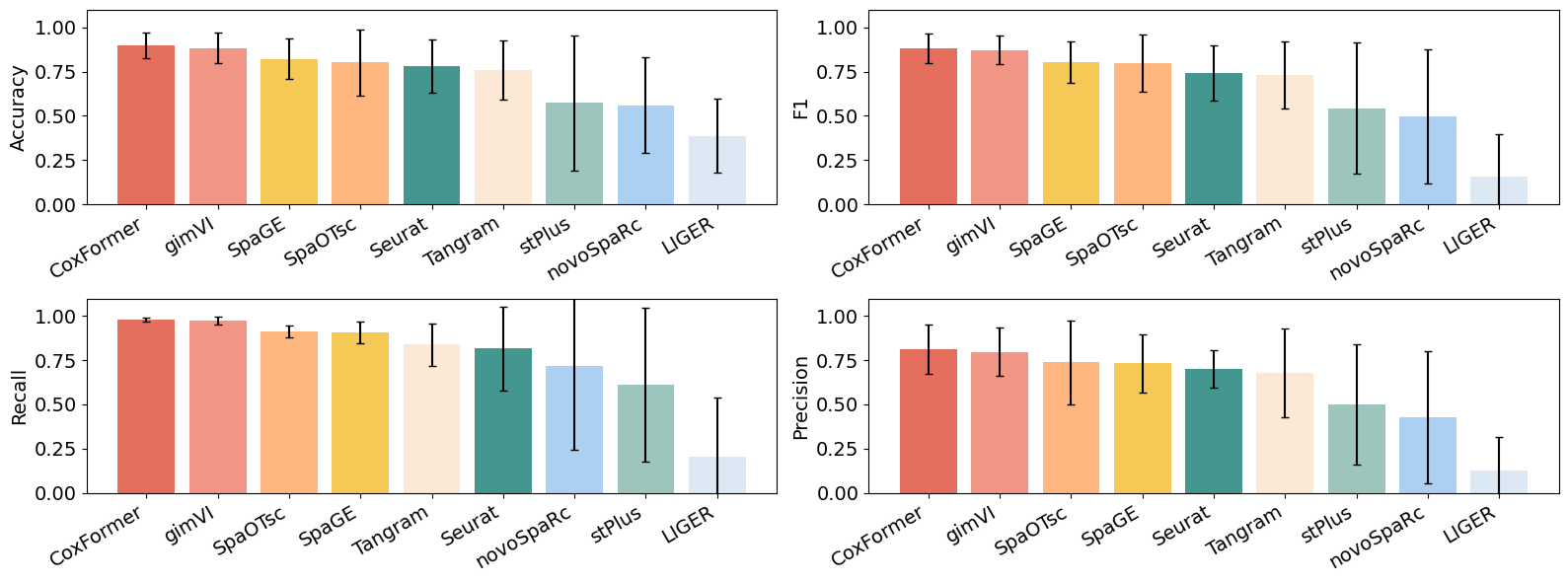
3.1 Barplots (mean ± std)

This subsection aggregates per-dataset metrics and visualizes mean ± standard deviation across datasets for standard metrics such as:

• Accuracy

• F1 score

• Recall

• Precision

Methods are plotted with a consistent color mapping to support direct comparison.

metrics = plot_metrics_barplots(RES_PATH, datasets, color_map, save=True)

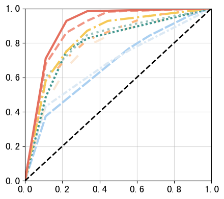
3.2 ROC plots (mean ROC across datasets)

This subsection computes and visualizes the mean ROC curve across datasets for each method.

Procedure:

1. Read the ROC points (fpr, tpr) from each dataset’s metrics.csv.

2. Interpolate TPR to a shared FPR grid.

3. Average the interpolated curves across datasets.

4. Plot the mean ROC curves using a consistent color scheme and line styles.

AUC values are displayed in the legend when available.

roc = plot_mean_roc(RES_PATH, datasets, color_map,save=False)

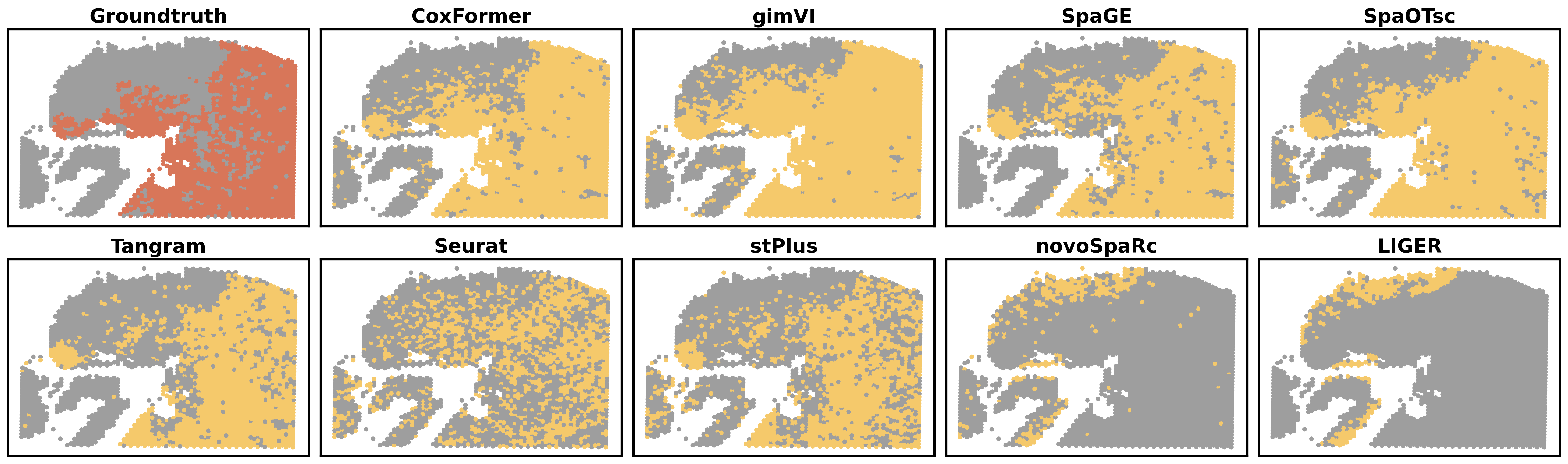
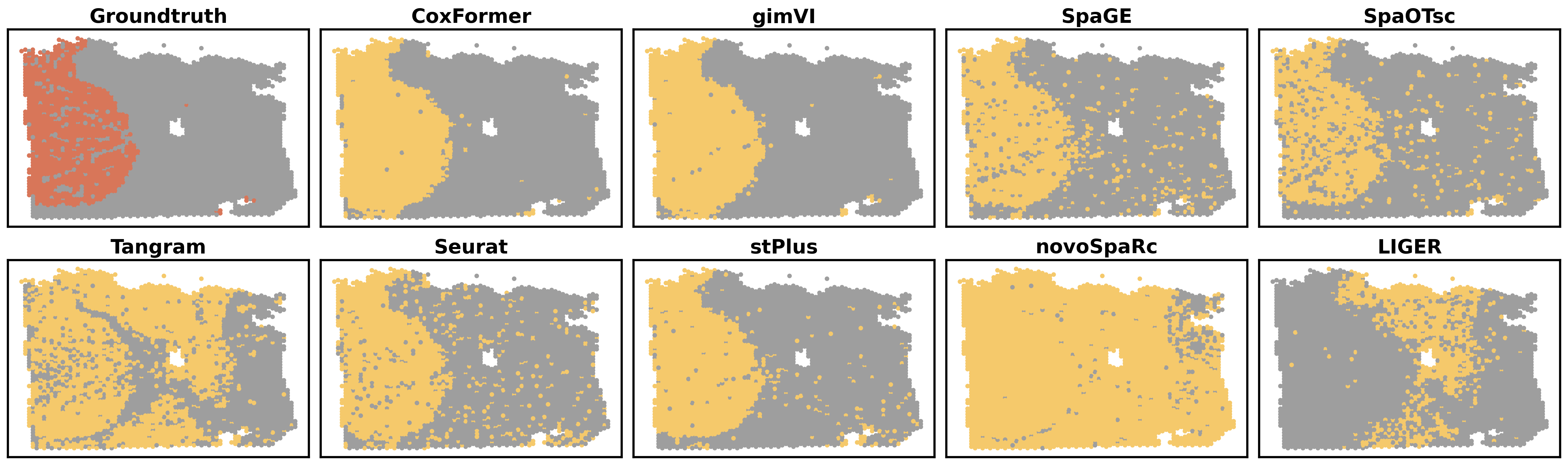
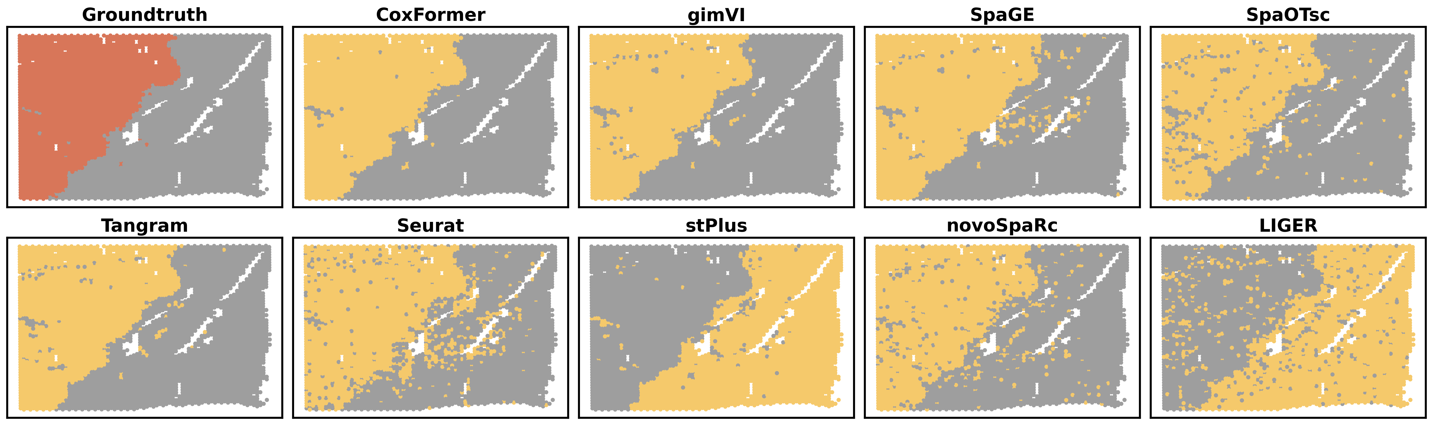
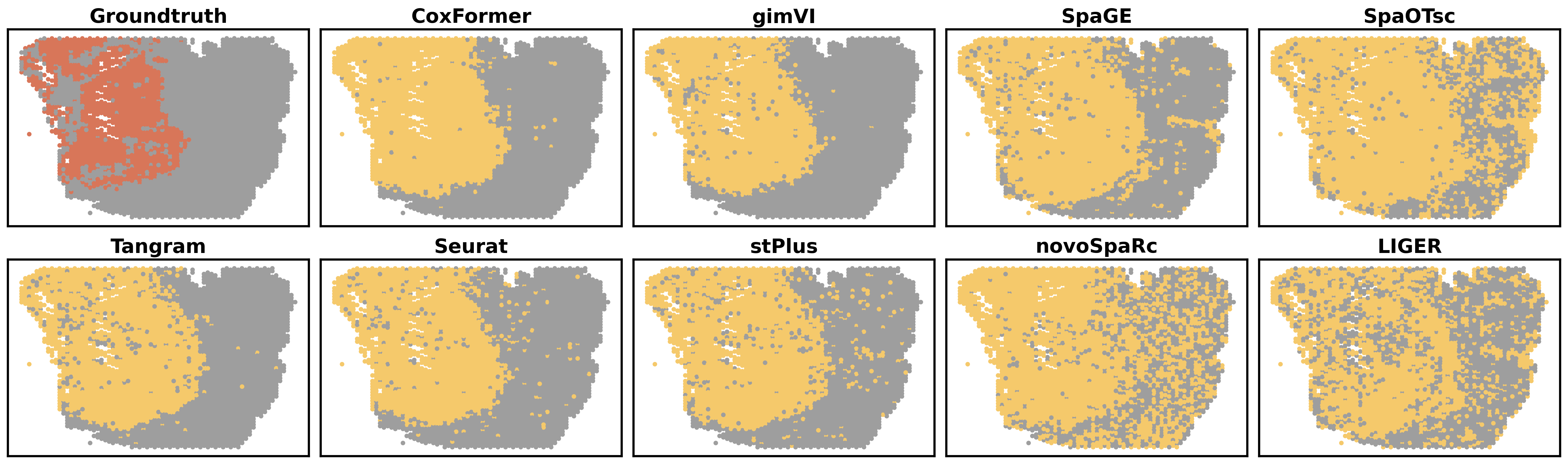
3.3 Abnormal-region spatial plots

This subsection visualizes abnormal-region predictions in the original tissue coordinate space.

• The reference spatial coordinates and ground-truth abnormal label are extracted from a reference AnnData file.

• For each method, a predicted abnormal region is derived from method-specific cluster assignments (e.g., Leiden clusters) using a deterministic rule (e.g., selecting the cluster with the highest mean absolute expression across genes).

The output is a multi-panel figure including the ground truth and method predictions.

for dataset in datasets:
    plot_abnormal_region(os.path.join(RES_PATH,dataset), dataset, methods)

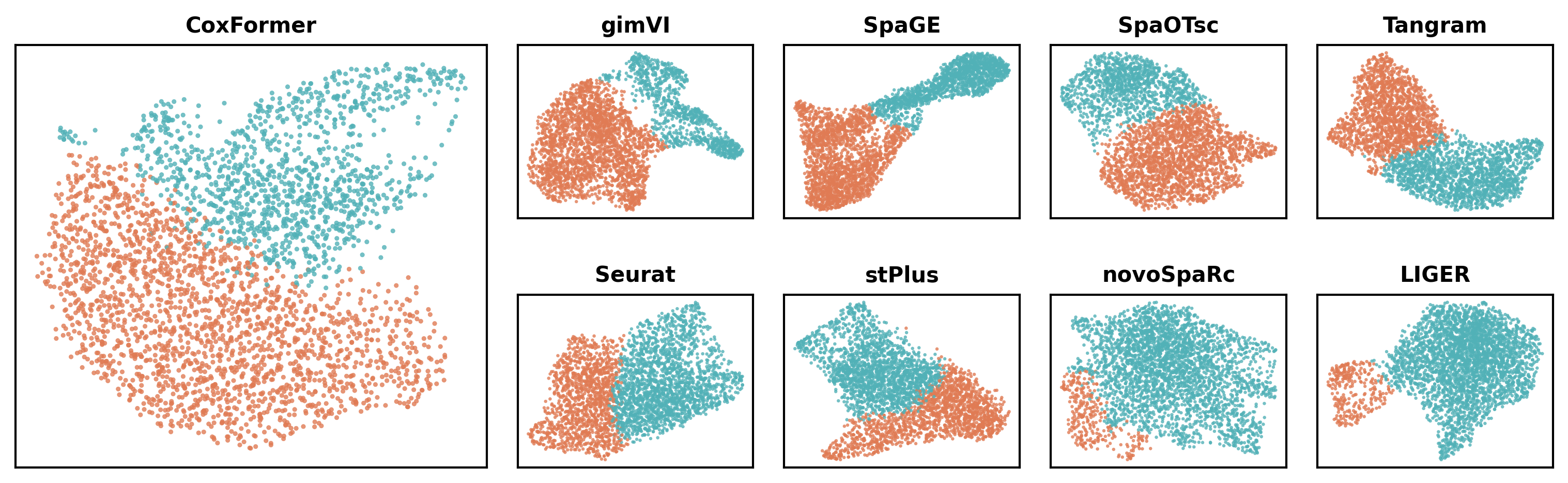
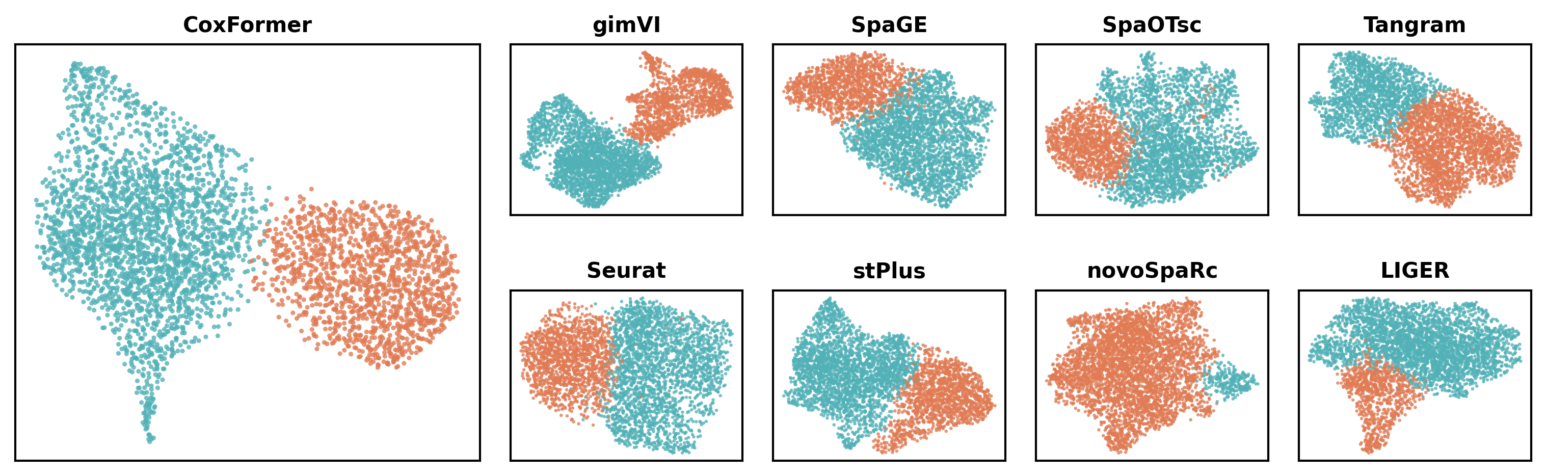
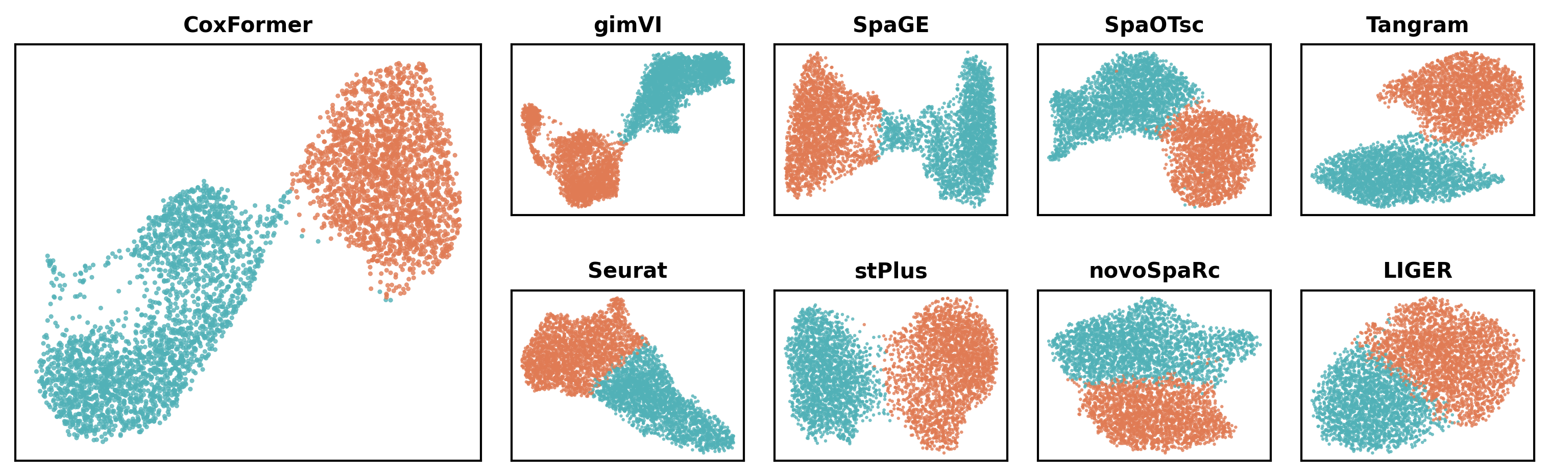
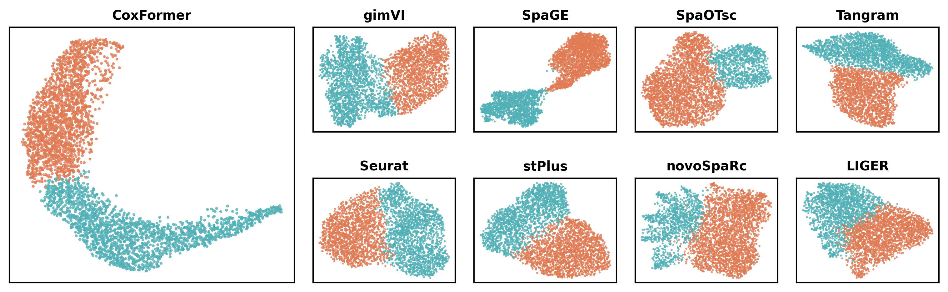
3.4 Abnormal-region UMAP plots

This subsection visualizes the clustering structure in a low-dimensional space.

For each method:

• Load the method-specific AnnData output (e.g., {Method}_deg.h5ad).

• Read the UMAP embedding (e.g., obsm["X_umap"]) and cluster labels (e.g., obs["leiden"]).

• Highlight the selected “abnormal-associated” cluster (defined using the same rule as the spatial plots) to show its separation in embedding space.

for dataset in datasets:
    plot_umap(os.path.join(RES_PATH,dataset), dataset, methods)

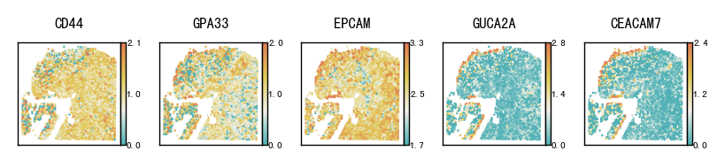
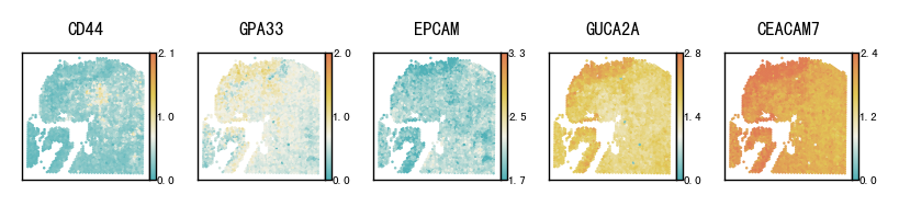
4 Selected marker genes spatial heatmap plot

This section visualizes the spatial patterns of a small set of marker genes. For each selected gene, spatial scatter plots are generated for:

• Ground truth

• CoxFormer imputation

The goal is to compare spatial structure and regional variation across methods under the same visualization settings.

colors = ["#51B1B7",'#F2F1E6','#E1C855', "#E07B54"]
cmap = mcolors.LinearSegmentedColormap.from_list("custom_cmap", colors)
dataset = "CRC1"
locs = pd.read_csv(os.path.join(DATA_PATH, dataset, "locs.tsv"), header=0, sep="\t", index_col=0)
groundtruth = pd.read_csv(os.path.join(RES_PATH,dataset,"groundtruth.csv"), sep=",")
coxformer = pd.read_csv(os.path.join(RES_PATH,dataset,'CoxFormer_impute.csv'),sep=',')
gene_show = ['CD44','GPA33','EPCAM','GUCA2A',"CEACAM7"]
plot_gene_spatial(gene_show, locs, {"Ground Truth": groundtruth, "CoxFormer": coxformer},
                  save_dir=os.path.join(RES_PATH,dataset), prefix="nhk", layout="pages",s=0.8,
                  ncols=5, per_ax=0.8, cmap=cmap, add_colorbar=True)

Result/Pathological_region_detection/CRC1/nhk_Ground_Truth.pdf already exists, skip saving.

Result/Pathological_region_detection/CRC1/nhk_CoxFormer.pdf already exists, skip saving.

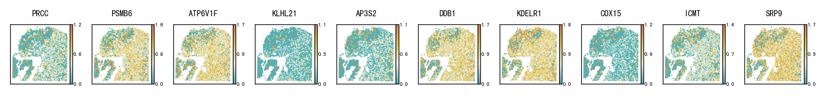
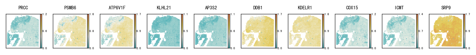
5 Selected housekeeping genes spatial heatmap plot

This section visualizes the spatial patterns of a small set of housekeeping genes. For each selected gene, spatial scatter plots are generated for:

• Ground truth

• CoxFormer imputation

The goal is to compare spatial structure and regional variation across methods under the same visualization settings.

colors = ["#51B1B7",'#F2F1E6','#E1C855', "#E07B54"]
cmap = mcolors.LinearSegmentedColormap.from_list("custom_cmap", colors)
dataset = "CRC1"
locs = pd.read_csv(os.path.join(DATA_PATH, dataset, "locs.tsv"), header=0, sep="\t", index_col=0)
groundtruth = pd.read_csv(os.path.join(RES_PATH,dataset,"groundtruth.csv"), sep=",")
coxformer = pd.read_csv(os.path.join(RES_PATH,dataset,'CoxFormer_impute.csv'),sep=',')
gene_show = ['PRCC','PSMB6','ATP6V1F','KLHL21','AP3S2','DDB1','KDELR1','COX15','ICMT','SRP9']
plot_gene_spatial(gene_show, locs, {"Ground Truth": groundtruth, "CoxFormer": coxformer},
                  save_dir=os.path.join(RES_PATH,dataset), prefix="hk", layout="pages",s=0.8,
                  ncols=10, per_ax=0.8, cmap=cmap, add_colorbar=True)

Result/Pathological_region_detection/CRC1/hk_Ground_Truth.pdf already exists, skip saving.

Result/Pathological_region_detection/CRC1/hk_CoxFormer.pdf already exists, skip saving.

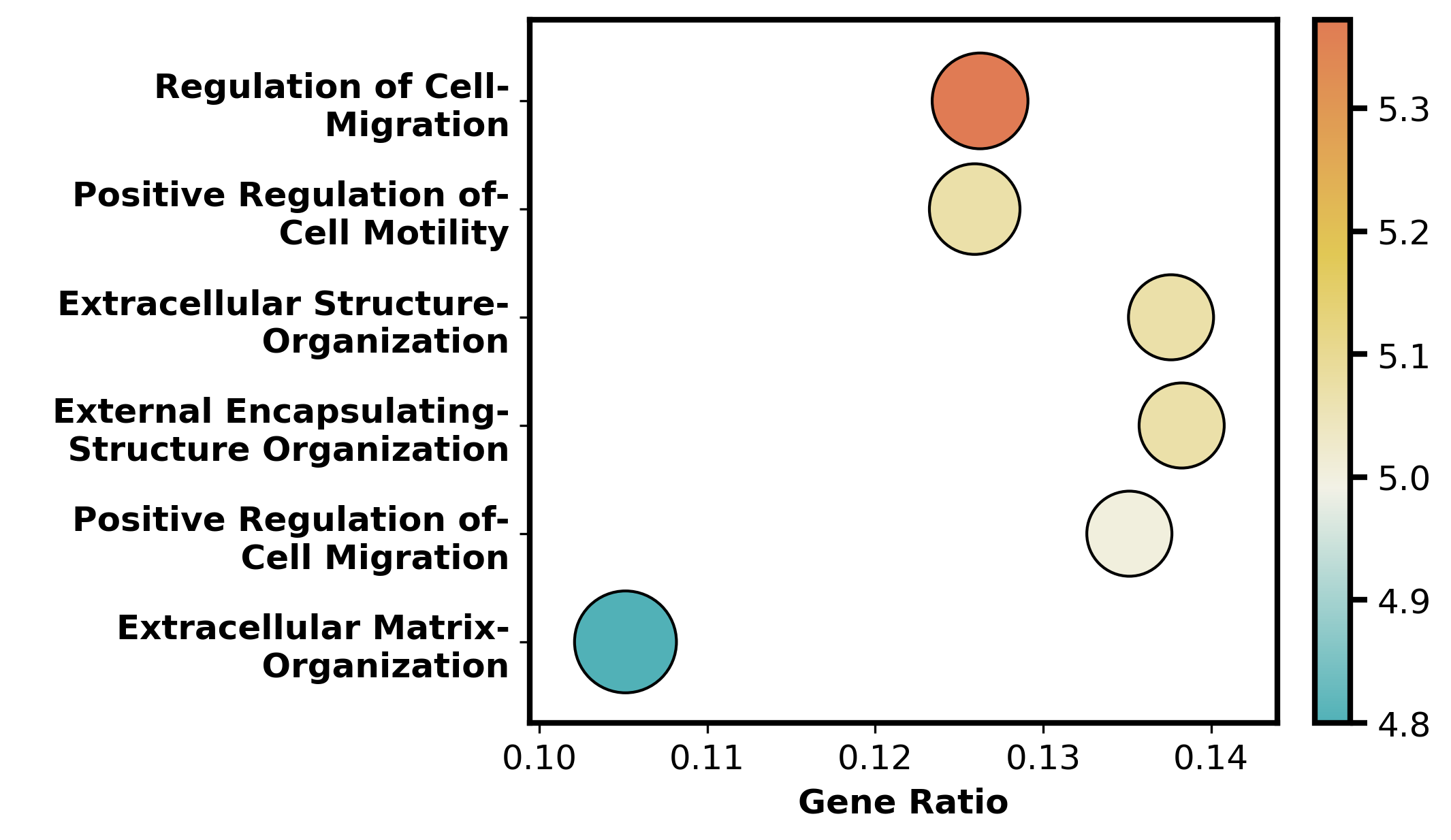
6 GO enrichment analysis

colors = ["#51B1B7",'#F2F1E6','#E1C855', "#E07B54"]
cmap = mcolors.LinearSegmentedColormap.from_list("custom_cmap", colors)
dataset = "CRC1"
glist = np.load(os.path.join(RES_PATH,dataset,f"{dataset}_CoxFormer_deg_list.npy"),allow_pickle=True)
dfb, score, score_label = GO_analysis(glist)
fig, ax = plt.subplots(figsize=(7, 4), dpi=300, constrained_layout=True)
plot_go_bubble(ax, dfb, "GO Biological Process Enrichment",cmap)
plt.show()

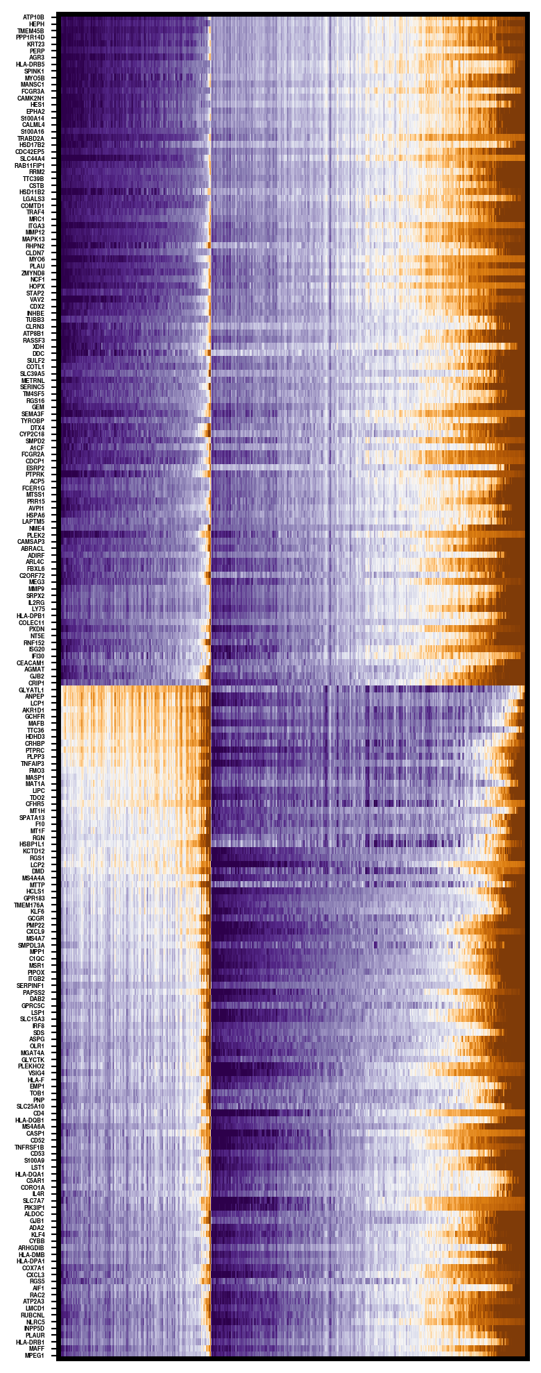
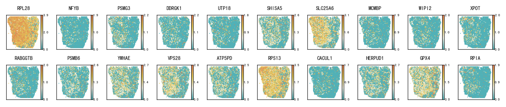
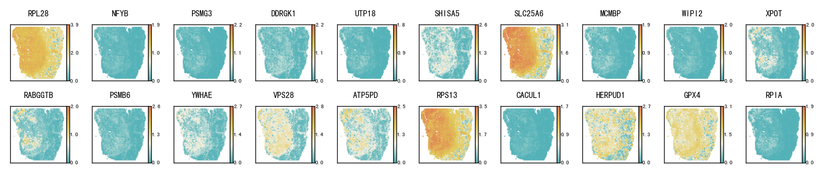
7 Supplementary

colors = ["#51B1B7",'#F2F1E6','#E1C855', "#E07B54"]
cmap = mcolors.LinearSegmentedColormap.from_list("custom_cmap", colors)
dataset = "LM2"
locs = pd.read_csv(os.path.join(DATA_PATH, dataset, "locs.tsv"), header=0, sep="\t", index_col=0)
groundtruth = pd.read_csv(os.path.join(RES_PATH,dataset,"groundtruth.csv"), sep=",")
coxformer = pd.read_csv(os.path.join(RES_PATH,dataset,'CoxFormer_impute.csv'),sep=',')
gene_show = [
    "RPL28","NFYB","PSMG3","DDRGK1","UTP18","SHISA5","SLC25A6",
    "MCMBP","WIPI2","XPOT","RABGGTB","PSMB6","YWHAE","VPS28","ATP5PD",
    "RPS13","CACUL1","HERPUD1","GPX4","RPIA"
]
plot_gene_spatial(gene_show, locs, {"Ground Truth": groundtruth, "CoxFormer": coxformer},
                  save_dir=os.path.join(RES_PATH,dataset), prefix=f"{dataset}_hk", layout="pages",s=0.8,
                  ncols=10, per_ax=0.8, cmap=cmap, add_colorbar=True)

Result/Pathological_region_detection/LM2/LM2_hk_Ground_Truth.pdf already exists, skip saving.

Result/Pathological_region_detection/LM2/LM2_hk_CoxFormer.pdf already exists, skip saving.

adata_imp = sc.read_h5ad(os.path.join(RES_PATH,dataset, f"{dataset}_CoxFormer_deg.h5ad"))
truth_column = "ident.annot"
s = adata_imp.obs[truth_column].astype(str)
adata_imp.obs['region'] = pd.Categorical(
    np.where(s.eq('Tumor'), 'Tumor', 'Other'),
    categories=['Other', 'Tumor']
)
label = adata_imp.obs['region']
label = label.reset_index(drop=True)
markers, genes_show = get_topk_markers(coxformer[adata_imp.var.index], label, topk=100,clusters=['Tumor','Other'])
ordered_spots = order_spots_by_marker_score(coxformer[adata_imp.var.index], label, markers, ['Tumor','Other'])
coxformer_hm  = coxformer.loc[ordered_spots, genes_show]
fig, ax = plt.subplots(1, 1, figsize=(4, 10), dpi=200)
plot_gaussian_heatmap(ax, coxformer_hm, vmin=None, vmax=None, cmap='PuOr',show_ticks=True,fontsize=3)
plt.tight_layout()
plt.show()