Gene Activity Score Prediction Tutorial (Hippocampus)

This tutorial evaluates ATAC accessibility imputation on the Hippocampus dataset by comparing the ground truth matrix to CoxFormer imputed results.

The notebook includes:

• Metric computation and a radar summary across methods (e.g., PCC, SSIM, RMSE).

• Spatial visualization of selected genes to compare spatial patterns between ground truth and imputations.

• Spatial annotation of ATAC clusters (e.g., CA3 and GCL) for regional context.

• DEG heatmap analysis for predefined regions (CA3 vs GCL) with shared color scaling across methods.

All functions are available in utils/.

0. Configuration

Define the dataset module (e.g., Hippocampus) and set the paths:

• DATA_PATH: input data directory (e.g., meta.tsv, cnts.tsv, locs.tsv)

• RES_PATH: imputation results and evaluation outputs (e.g., {tool}_impute.csv, {tool}_Metrics.txt)

## import packages
import os
import pandas as pd
import matplotlib.pyplot as plt
os.chdir(os.path.abspath(".."))
from utils.Gene_expression_prediction_utils import CalDataMetric
from utils.Gene_activity_score_prediction_utils import plot_radar, plot_atac_spatial, plot_spatial_scatter, plot_cluster_heatmaps

dataset = "Hippocampus"
RES_PATH  = f"Result/Gene_activity_score_prediction/{dataset}/"
DATA_PATH = f"Dataset/Gene_activity_score_prediction/{dataset}/"

1. Load ground truth and imputed matrices

This section loads:

• meta.tsv: spot-level metadata (e.g., cluster labels and optional pseudotime)

• cnts.tsv: ground truth gene activity scores matrix (genes × score)

• {tool}_impute.csv: imputed ATAC matrices from different methods

meta = pd.read_csv(os.path.join(DATA_PATH, "meta.tsv"), sep="\t", header=0, index_col=0)
gt   = pd.read_csv(os.path.join(DATA_PATH, "cnts.tsv"), sep="\t", header=0, index_col=0)
location = pd.read_csv(os.path.join(DATA_PATH, "locs.tsv"), header=0, index_col=0, sep="\t")

impute_our = pd.read_csv(os.path.join(RES_PATH, "CoxFormer-Loc_impute.csv"), header=0).set_axis(gt.index, axis=0)
impute_cor = pd.read_csv(os.path.join(RES_PATH, "correlation_pca-Loc_impute.csv"), header=0).set_axis(gt.index, axis=0)
impute_cox = pd.read_csv(os.path.join(RES_PATH, "coexpression_pca-Loc_impute.csv"), header=0).set_axis(gt.index, axis=0)
impute_txt = pd.read_csv(os.path.join(RES_PATH, "text-Loc_impute.csv"), header=0).set_axis(gt.index, axis=0)

1.1 Metric computation

This section calls CalDataMetric(...) to compute evaluation metrics for imputation quality and writes results to RES_PATH (e.g., {tool}_Metrics.txt).

Example metrics:

• PCC and SSIM: higher values indicate better agreement with ground truth.

• RMSE: lower values indicate smaller reconstruction error.

CalDataMetric(RES_PATH, os.path.join(DATA_PATH, "cnts.tsv"))

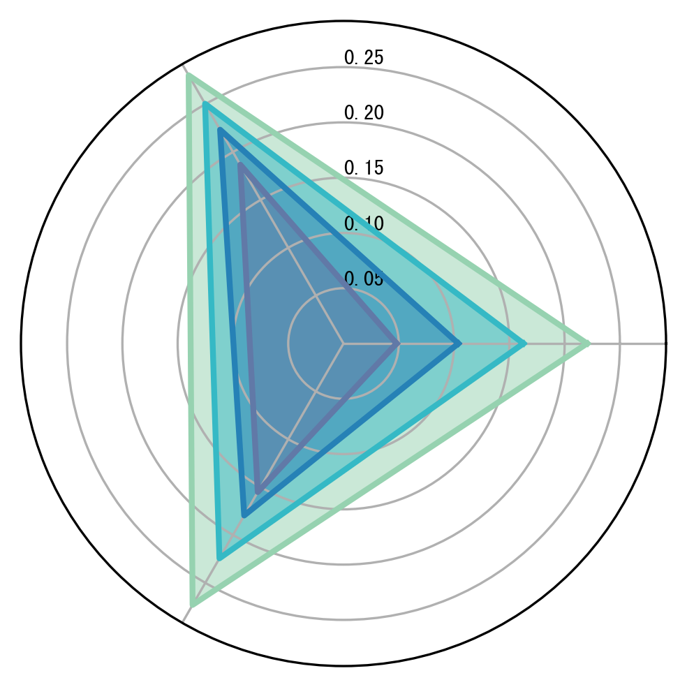
1.2 Radar summary of metrics

This section reads {tool}_Metrics.txt for each method and summarizes the mean metric values across features. A radar plot is used to provide a compact comparison across methods.

Note: RMSE apply a consistent transformation before plotting to avoid misinterpretation.

metric = ['PCC', 'SSIM', 'RMSE']
colors = ["#96D2B0","#35B9C5","#2681B6","#6179A7"]
Tools = ['CoxFormer-Loc',"coexpression_pca-Loc","correlation_pca-Loc","text-Loc"]
plot_radar(RES_PATH, metric, Tools, colors, save=False)

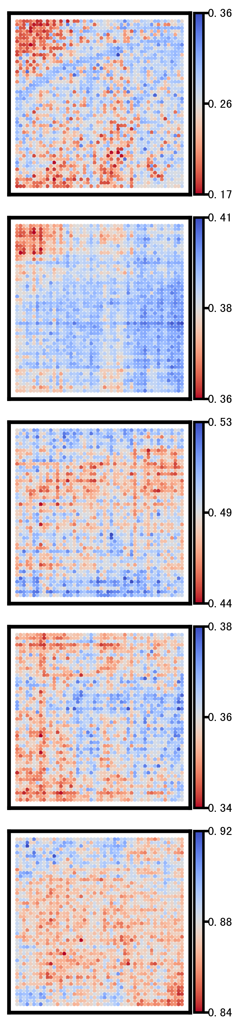
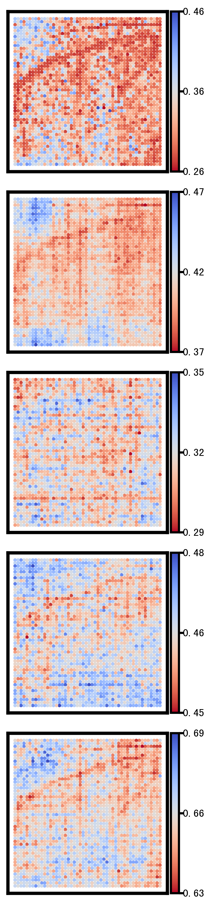
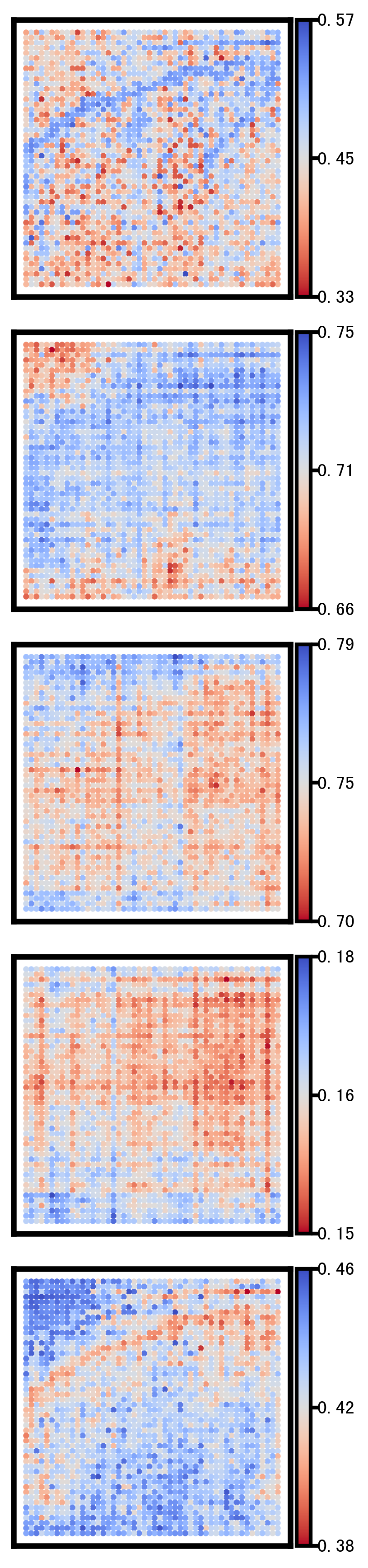
2 Selected genes spatial heatmap plot

This section visualizes the spatial patterns of a small set of representative genes. For each selected gene, spatial scatter plots are generated for:

• Ground truth

• CoxFormer imputation

• Co-expression imputation

• Correlation imputation

• Description imputation

The goal is to compare spatial structure and regional variation across methods under the same visualization settings.

Selected_list = ['SMIM27','SMDT1','BIN2','ASAH1','NPAS4']
data = {
    "GroundTruth": gt,
    "CoxFormer": impute_our,
    "Coexpression": impute_cox,
    "Correlation": impute_cor,
    "Description":impute_txt,
}
plot_atac_spatial(
    gene_list=Selected_list,
    location=location,
    data=data,
    save_dir=RES_PATH,
    add_colorbar=True,
    s=10,
    methods=("GroundTruth", "CoxFormer", "Coexpression","Correlation","Description"),
)

Gene: SMIM27

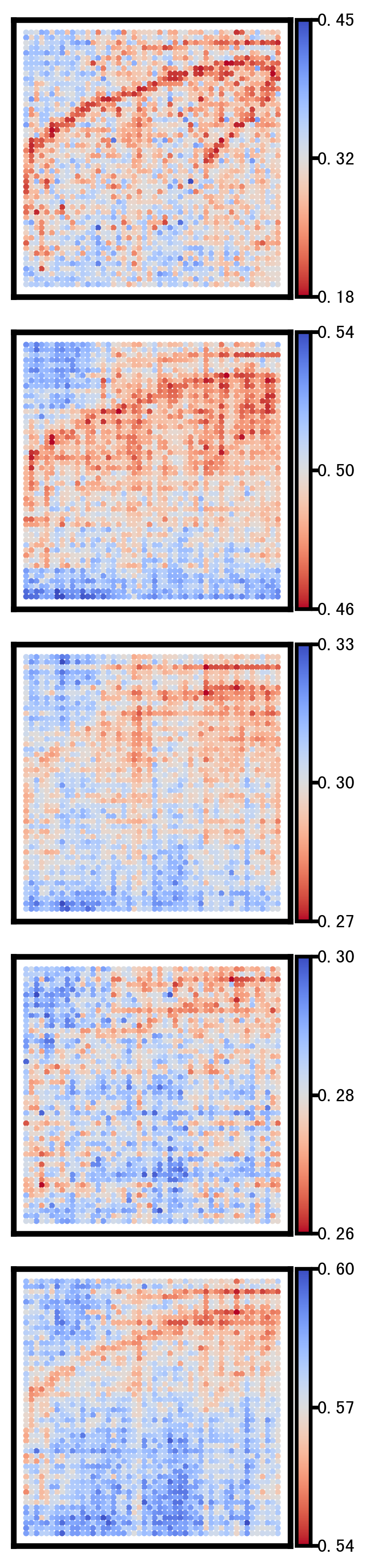
Gene: SMDT1

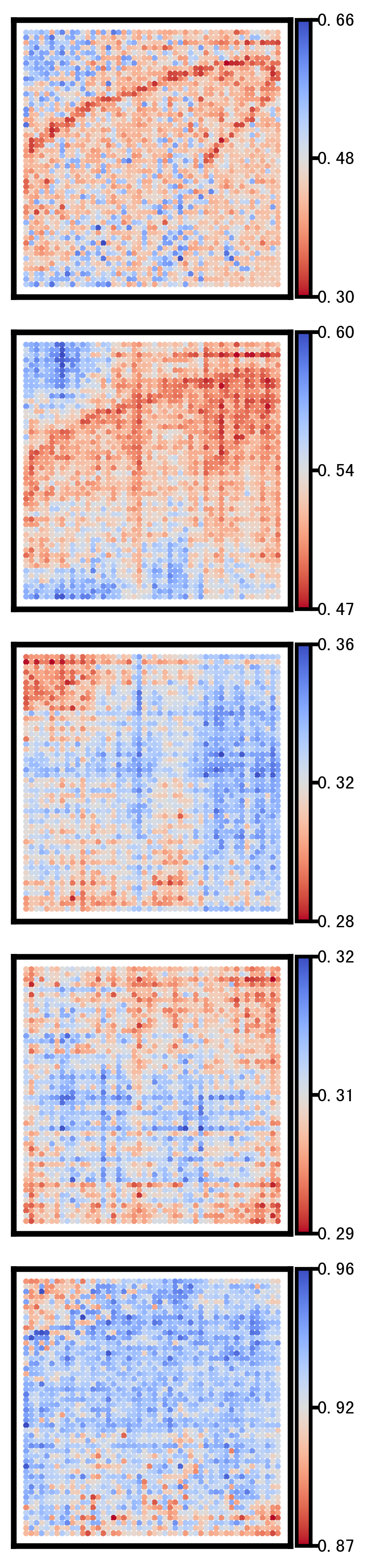
Gene: BIN2

Gene: ASAH1

Gene: NPAS4

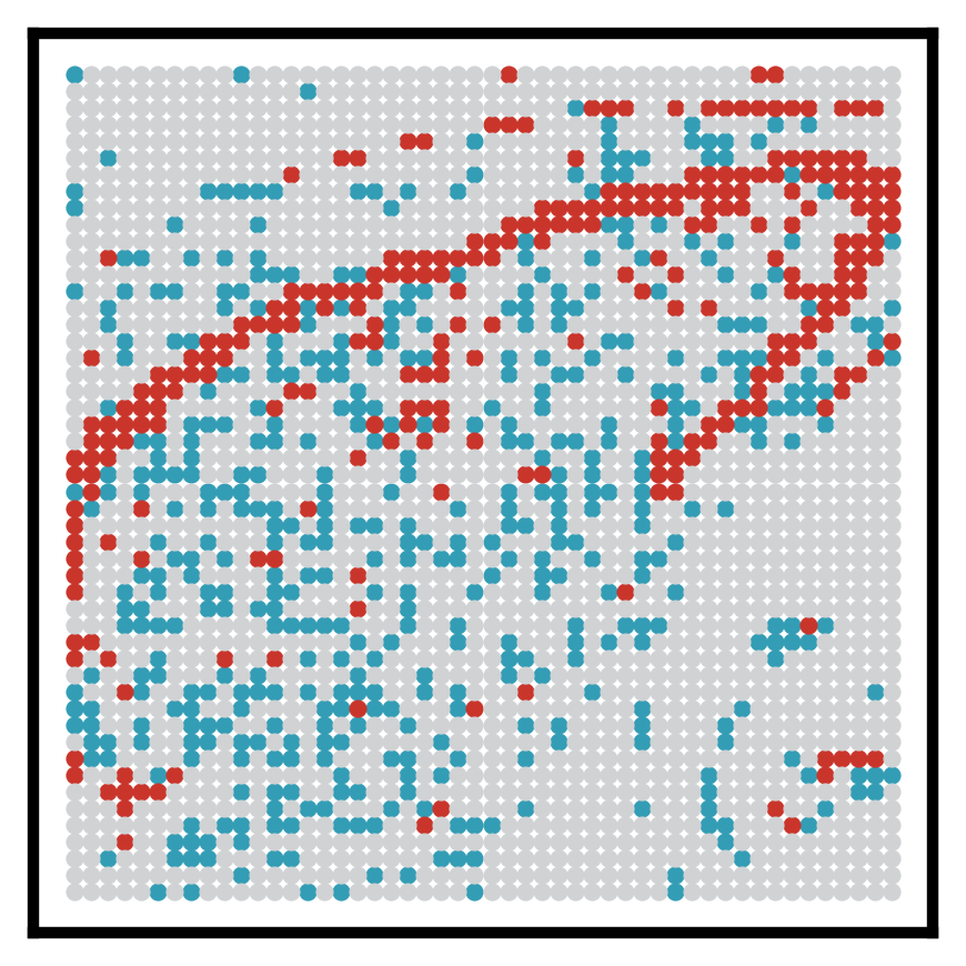
3. Visualize spatial ATAC clusters

This section visualizes cluster annotations from meta["ATAC_clusters"] in spatial coordinates. Cluster labels are optionally mapped to more interpretable region names (e.g., CA3 and GCL), with all remaining labels grouped as “Other”.

This plot provides spatial context for region-specific analyses performed in later sections.

name_map = {"C1": "CA3 pyramidal layer (CA3 Pyr)", "C4": "Granule cell layer (DG GCL)"}
color_map = {"CA3 pyramidal layer (CA3 Pyr)": "#339DB5",
             "Granule cell layer (DG GCL)"  : "#C9352B",
             "Other"                        : "#D0D2D4"}

cluster_series = meta["ATAC_clusters"].reindex(location.index).map(name_map).fillna("Other")
fig, ax = plt.subplots(1, 1, figsize=(3, 3), dpi=300)
plot_spatial_scatter(ax, location, cluster_series, mode="categorical",
             color_map=color_map,add_legend=False, s=15)
plt.tight_layout()
plt.show()

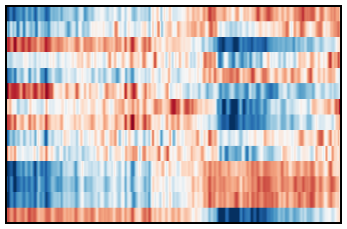
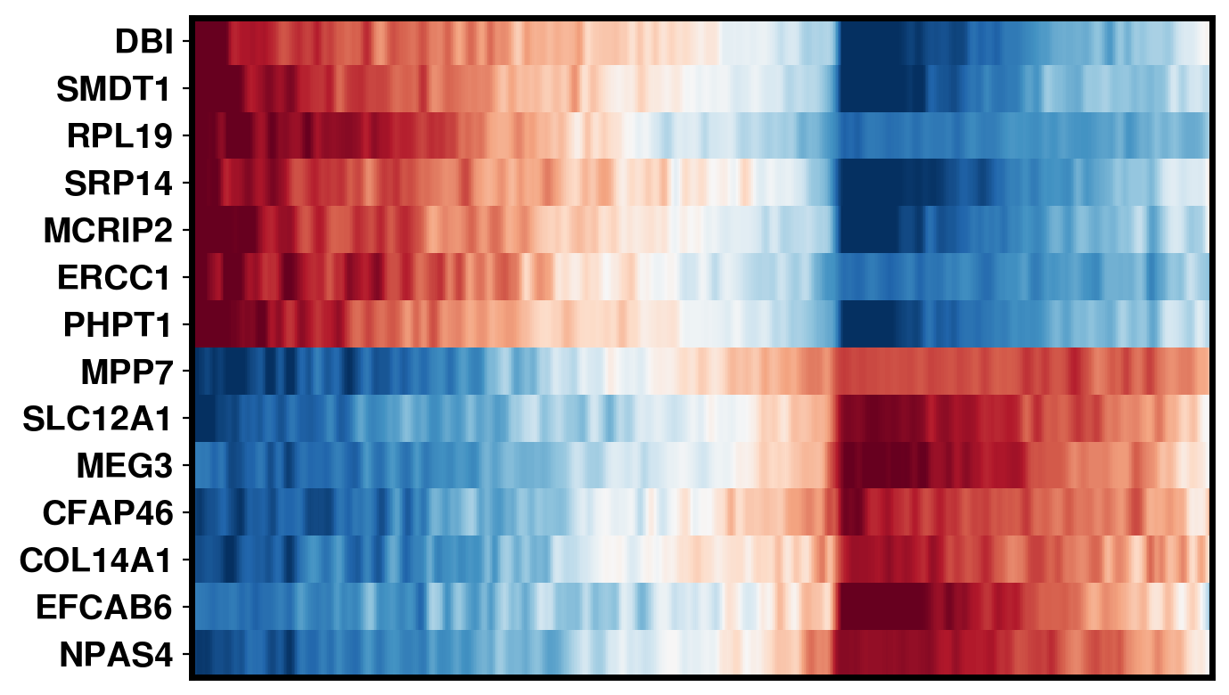
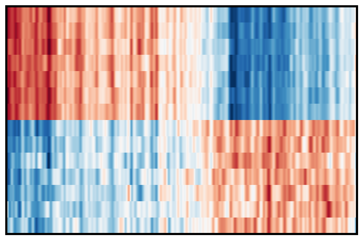
4. Plot DEG of defined cluster

This section compares region-specific accessibility patterns between CA3 and GCL:

1. Align shared features across ground truth and imputed matrices.

2. Subset spots to CA3 and GCL based on metadata labels.

3. For each region, perform a Wilcoxon-based differential analysis to identify top marker features (topK).

4. Order spots within each region using the mean accessibility of region-specific markers.

5. Plot heatmaps for ground truth, CoxFormer, Co-expression, Correlation and Description using a shared color scale (derived from ground truth).

This provides a direct visual comparison of region-specific signal patterns across methods.

data = {
    "GroundTruth": gt,
    "CoxFormer": impute_our,
    "Coexpression": impute_cox,
    "Correlation": impute_cor,
    "Description":impute_txt,
}
plot_cluster_heatmaps(data=data,meta=meta, clusters=["CA3", "GCL"],RES_PATH=RES_PATH)

Ground Truth:

CoxFormer:

Coexpression:

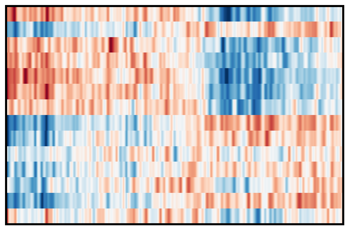
Correlation:

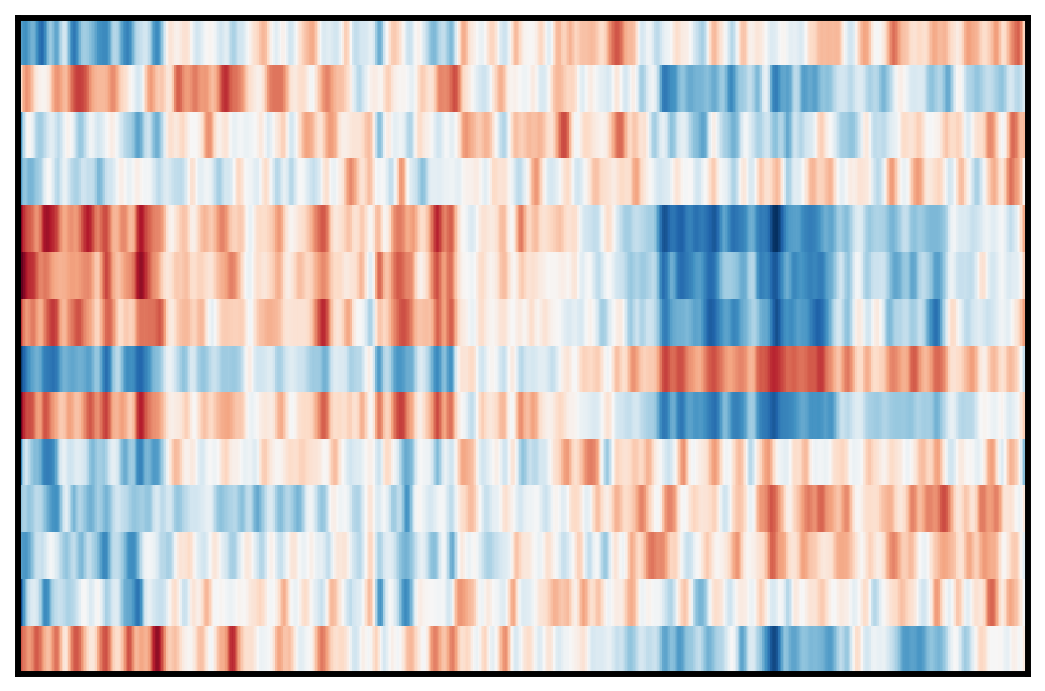
Description: